From Words to Waypoints: Teaching a Small LLM to Plan for Robots
Large language models are increasingly asked to act as the high-level planner of a robot: given a task in words or in a formal language, decide where to go, in which order, and when. For tasks written in temporal logic, the classical approach is to encode the whole problem as a mixed-integer linear program (MILP) and hand it to a solver. That works, but it can take a very long time, and the cost grows quickly with the length of the task and the number of conditions. A MILP solver is a powerful but blind search: every operator, at every time step, becomes a set of binary variables and constraints, and the solver has no notion of what they mean. A language model can understand the semantics of the temporal operators, for instance that “stay out of D until K is reached” means visiting K before entering D, and use common sense to come up with a plan directly. This post does not compare the two approaches rigorously, and we have no evidence that an LLM planner is better than a MILP solver; we are showing that the LLM route is possible.
We wanted to know whether a small open model can learn to do this well. Concretely, the goal was to take Qwen3.5-9B and train it with reinforcement learning until it solves robot planning tasks written in temporal logic about as reliably as a much larger model, DeepSeek-V4.1-Flash-1017, which we use as the reference (“the teacher”).
This post tells the story of how we got there, in the order it happened: a first attempt that learned nothing, the fix that made learning possible, and the step that made it fast.
The problem
A robot moves in a 2D workspace with rectangular obstacles and named regions. Its task is a specification in Signal Temporal Logic (STL), a language for properties of trajectories over time.The setting follows Multi-agent Motion Planning from Signal Temporal Logic Specifications, restricted to one robot with a speed limit. Any feasible path is accepted; we do not ask for the optimal one. A specification combines two kinds of pieces. Atoms say where the robot is: in(B) holds when the robot is inside region B, and out(A) when it is outside region A, where A, B, K, D and Goal are names of regions on the map. Temporal operators say when an atom has to hold. They are written as single capital letters followed by a time window in seconds: F means “eventually” (at some time in the window), G means “always” (at every time in the window), and p U q means “p holds until q does”. Operators can be nested, as in the last example. Below are some examples of STL specifications:
F[7,21] in(B): be inside region B at some time between 7 and 21 seconds;G[0,30] out(A): stay out of region A for the first 30 seconds;out(D) U[0,136] in(K): stay out of D until K is reached, within 136 seconds;F[153,169] G[0,5] in(Goal): at some time between 153 and 169, enter the goal and stay there for 5 seconds.
The model reads the map and a list of such clauses and must answer with a timed path, a list of waypoints [[t, x, y], ...]. The robot is a small square that must never touch an obstacle and cannot move faster than its speed limit.
Everything the model knows about the task comes from its prompt. The system prompt explains the robot and path model, defines the STL atoms and operators with a couple of examples, and fixes the answer format; the user message lists the workspace, every obstacle and region as coordinates, the robot’s size, speed limit and start, and the specification clauses. There are no solved examples in the prompt, and every model in this post, the teacher included, gets the same prompt.
The full system prompt
You are a high-level motion planner for a single mobile robot in a 2D workspace. Your job is to produce a timed path for the robot that satisfies a Signal Temporal Logic (STL) specification. Any feasible path is accepted; it does not need to be optimal.

# Robot and path model
- The robot is an axis-aligned square with half-width r: at position (x, y) its body occupies [x-r, x+r] x [y-r, y+r]. It translates only (no rotation).
- A path is a list of waypoints [[t0, x0, y0], [t1, x1, y1], ...] with t0 = 0 and (x0, y0) = the start position. Times must be non-decreasing.
- Between consecutive waypoints the robot moves in a straight line at constant speed. The speed on each segment, distance / (t_{k+1} - t_k), must not exceed v_max. To wait, repeat the same position at a later time.
- After the last waypoint the robot stays there forever.
- The robot body must always stay inside the workspace and must never overlap any obstacle (touching the boundary is fine).

# STL specification
All regions are axis-aligned rectangles. Atomic propositions:
- in(R): the robot body is fully inside region R (equivalently, x in [xmin+r, xmax-r] and y in [ymin+r, ymax-r]).
- out(R): the robot body is fully outside region R (it does not overlap R).
Operators (a, b are absolute durations in seconds, measured from the time the formula is evaluated):
- p & q: both hold.  p | q: at least one holds.
- F[a,b] p ("eventually"): p holds at some time in [t+a, t+b].
- G[a,b] p ("always"): p holds at every time in [t+a, t+b].
- p U[a,b] q ("until"): q holds at some time t' in [t+a, t+b], and p holds at every time in [t, t'].
Formulas can be nested, e.g. F[0,30] G[0,5] in(A) means "at some time t in [0,30], enter A and stay in A for 5 seconds (during [t, t+5])"; G[0,50] F[0,20] in(B) means "during [0,50], B is always visited again within 20 seconds".
The whole specification is evaluated at time t = 0, and every listed item (phi1, phi2, ...) must hold.
# Planning
You have no tools. Reason carefully about geometry (stay clear of obstacles, using corner points at least r away from them) and timing (respect v_max), then give the final answer.
# Final answer
When you are done, write the final path inside <answer></answer> tags as a JSON list of [t, x, y] waypoints, e.g.
<answer>[[0, 1.0, 1.0], [5.2, 4.0, 3.5], [9, 4.0, 3.5]]</answer>
Only the last <answer> block in your final message is graded. The answer is correct only if the path is feasible and satisfies every specification item.
A planning task like this is a good fit for RL because the answer can be checked exactly. Our checker computes, for a piecewise-linear path and rectangular regions, the exact set of times at which each atom holds, and evaluates the temporal operators on those interval sets, so there is no sampling error. The reward is 1 if the path is collision-free, respects the speed limit and satisfies every clause, and 0 otherwise.
Building the environment
An RL environment needs a stream of tasks that are solvable, checkable, and of the right difficulty. We generate them path first: the generator draws a map, picks a plan (an order of region visits, waits, dwell times, regions to keep away from), builds a path for that plan, and only then derives the STL clauses from the path’s actual timing, with randomized slack in the time windows. Every instance therefore has a known solution. The generator also runs a naive baseline (visit the regions in order, no waiting, no avoidance) and resamples most instances that the baseline already solves, so that the clauses actually interact.
The instances come in eight levels, meant as the rungs of a ladder:
| level | map | specification |
|---|---|---|
| L1 | room, 3–6 obstacles | 2–3 timed visits, one region to avoid throughout |
| L2 | room, 4–8 obstacles | visits, holds, until, choices, avoid windows; 3–5 clauses |
| L3 | room, 4–8 obstacles | adds sequences and patrols, nesting depth 2, tight windows; up to 7 clauses |
| L4 | maze, 4–6 cells a side | as L2 |
| L5 | maze, 5–7 cells a side | as L3 |
| L6 | key-door maze, 1–2 doors | collect keys before crossing their doors, then reach the goal |
| L7 | key-door maze, 3–4 doors | nested keys (keys behind other doors) |
| L8 | key-door maze, 5–6 doors | as L7, at the scale of the hardest benchmarks in the paper above |
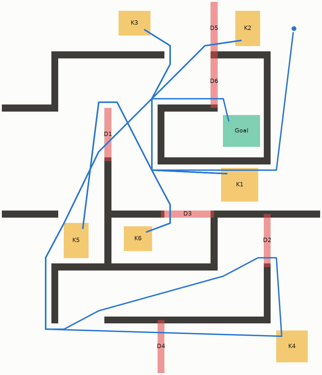
out(Doori) U[0,136] in(Keyi) clause per pair and F[153,169] G[0,5] in(Goal). Finding a feasible unlock order is the hard part.Why a ladder? We train with GRPO, which samples several answers per task (eight, in our case) and reinforces the ones that scored above the group’s average. If all eight fail, or all eight succeed, every answer gets the same score and the task contributes nothing to learning. The policy has to succeed sometimes. A ladder of levels makes it likely that some rung sits in that zone for the current model, both across the instances of a level and across the eight samples of one instance.
For evaluation we hold out 550 instances (50 each from L1–L7 and 200 from L8) and sample one answer per instance. On this set the teacher scores 0.90 overall and 0.80 on L8. The RL setup stays the same throughout the story: in every step we take 32 training tasks, half of them from L8, sample eight answers for each, and give each answer at most 32k tokens.More details: GRPO with the clip-higher trick from DAPO (0.2/0.28), no KL penalty, token-mean loss, LoRA rank 64 on all linear layers, learning rate 1e-5, up to 40 assistant turns per episode, trained with verl.
Attempt 1: plain RL
The first thing we tried was the simplest: give the base model the task and let RL do the rest. The model reasons in text and writes down the path.
It learned nothing. At the start, the base model solved 28% of L1, 24% of L2, 6% of L3 and essentially nothing from L4 upwards (0.06 overall). After 28 RL steps the training reward was still between 0.00 and 0.04, and the evaluation had not moved (0.062, 0.044 and 0.045 at steps 0, 10 and 20). In the first five steps, every group of eight samples on L5, L7 and L8 failed completely, and so did 86% of the groups on L3. The ladder we had built did not exist for this model: almost every rung was out of reach, so there was nothing to reinforce.
Why does it fail? Let us look at an example. In this L2 task the robot must wait in region E for a while, then reach region A without passing through region H, and later come back to E. The model writes almost 500 lines of reasoning; here is some of the model’s response where it works out the path:
- Distance: √((17.8-17.3)² + (13.3-6.5)²) = √(0.25 + 46.24) = √46.49 ≈ 6.82.
- Stay in E from t=6.82 to t=13.82. Duration 7s.
...
- Dist d1 = √((17.8-12.0)² + (13.3-17.9)²) = √(33.64 + 21.16) = √54.8 ≈ 7.40?
- (Previous rough calc was 4.67, mistake in distance estimation).
...
- Segment 3: E (17.3, 6.5) → Point U (17.3, 17.9).
  - X is constant 17.3. 17.3 > 15.3. Always out(H). Good.
- E → U: d = 11.4. Time 11.4. Arrive 13.82 + 11.4 = 25.22.
...
<answer>[[0, 17.8, 13.3], [6.82, 17.3, 6.5], [13.82, 17.3, 6.5], [25.22, 17.3, 17.9], ...]</answer>
The checker rejects the answer: one of the segments runs through an obstacle.
The response shows what goes wrong. The plan itself is right: wait in E, go around H, reach A in time. But the model then tries to turn the plan into numbers by itself, computing distances, arrival times and clearances by hand. It even catches one of its own arithmetic mistakes along the way, and still misses another one. LLMs make mistakes in this kind of calculation all the time, and one slip anywhere in a long chain of it is enough to make the whole path infeasible.
The example is typical. We sorted all 550 answers at step 0 by the first problem the checker found:
| outcome (550 test answers) | share |
|---|---|
| path goes through an obstacle | 79% |
| path is faster than the speed limit | 10% |
| answer missing or malformed | 3% |
| path is feasible but violates a clause | 1% |
| success | 6% |
Only 1% of the answers fail on the logic of the specification; almost all failures are calculation errors in the geometry or the timing.
So the model knows what to do but cannot compute the numbers, and RL cannot teach that from a reward that is almost always zero. We needed to give the model a calculator.
Attempt 2: give the model tools
We gave the model two tools:
plan_path(start, t_start, goal_region, avoid=[...], hold_until=...)returns the shortest collision-free path segment from a point to a region at full speed, optionally keeping out of some regions and waiting at the goal. It is complete: if it says there is no path, there is none.check_path(waypoints)runs the exact checker on a candidate path and explains what fails, for example'in(A)' never holds within [0, 38] (it holds at times: [41.2, 47]).
In the system prompt, the paragraph that told the model to work out the geometry by itself is replaced by a description of the tools and a suggested way to use them:
# Tools
You can call these tools (each call costs part of a limited budget):
- plan_path: computes the shortest collision-free path segment from a start point to a region or point, departing at a given time at maximum speed, optionally avoiding listed regions and optionally holding at the goal until a given time. Use it instead of computing geometry yourself.
- check_path: checks a full path and reports speed/collision/boundary violations and which specification items fail and why.
A good strategy: decide the order and timing of region visits that satisfies the specification, build the path segment by segment with plan_path (each segment starts where and when the previous one ended; insert waiting by choosing a later t_start or using hold_until), concatenate the waypoint lists, verify the full path with check_path, fix any reported problem, then give the final answer.
Both tools are fast. plan_path takes about 1–11 ms on average depending on the map (at most 37 ms on the largest mazes), and check_path at most 3 ms, so the exact geometry costs the model almost nothing, in contrast to solving the whole problem as a MILP.Why the gap is so large: the standard encoding of STL as a MILP (Raman et al., Model Predictive Control with Signal Temporal Logic Specifications, CDC 2014) introduces binary variables for every atom and every operator at every time step, and solving a MILP is NP-hard, so in the worst case the solver takes exponential time. AI has reportedly just refuted the Exponential Time Hypothesis, so maybe AGI will sort out the rest of complexity theory soon; we are hopeful, but until then an exponential is an exponential. plan_path solves a much easier problem, the shortest path for a square robot among rectangular obstacles. That is a shortest path on the visibility graph between obstacle corners, which takes polynomial time (roughly cubic in the number of obstacles in our simple implementation). The combinatorial part of the task, such as the order in which to collect the keys, does not go away; the language model handles it with common sense instead of exhaustive search, and without any guarantee.
The division of labor is the one the failure analysis suggests: the model decides what to do when (which region next, how long to wait, what to avoid), and the tools do the geometry, the timing and the verification. The final answer is still a list of waypoints, now usually the concatenation of the segments plan_path returned.
Thinking off. One setting dates from before the first attempt, but it is easiest to explain here. Qwen3.5 can run in a “thinking” mode, which writes a long hidden chain of thought before each reply. More reasoning sounds like the right thing for a planning task, so we measured both modes on the base model with these tools (30 tasks per level):This early test used a tighter setup than the main evaluation: each request reserved 16k tokens for the reply in a 32k context, so an episode ended as soon as the conversation passed about 16k tokens, and at most 24 turns. That is why its numbers are lower than those reported later. On the same 30 L8 tasks, the base model without thinking solves 5 here and 15 under the main evaluation’s 32k budget. Both modes ran under the same limits, but a tight budget penalizes the longer mode more; we did not repeat the comparison at 32k.
| base model | L1 | L2 | L3 | L4 | L5 | L6 | L7 | L8 | all | median tokens |
|---|---|---|---|---|---|---|---|---|---|---|
| thinking | 0.97 | 0.67 | 0.30 | 0.73 | 0.13 | 0.87 | 0.27 | 0.13 | 0.51 | 12.7k |
| no thinking | 0.93 | 0.77 | 0.50 | 0.87 | 0.23 | 0.93 | 0.37 | 0.17 | 0.60 | 7.4k |
Thinking was no better on any level except L1 (one task out of 30), clearly worse on L3 and L4, and used about 70% more tokens per episode. Its failures were mostly running out of room: 47% of its episodes ended without an answer, against 35% without thinking. We turned thinking off for every run in this post, the first attempt included; the model still reasons, in its visible reply.
With tools, the ladder appeared. The base model now solved 0.98 of L1, 0.92 of L2, 0.76 of L3, 0.92 of L4, 0.62 of L5, 0.94 of L6, 0.66 of L7 and 0.40 of L8 (0.67 overall). The easy levels were nearly solved, and L8 was hard but not hopeless.
Not every level is worth training on, though. In a preliminary study we trained on all levels equally, and the model soon solved almost every L1, L2, L4 and L6 task: 85–99% of its samples succeeded, against 20–60% on the other levels. Such tasks nearly always give groups where all eight samples succeed, which teach GRPO nothing, yet generating them costs as much as any other task. So we kept only a few of them and spent the training set on the hard levels, half of it on L8, the level furthest from the teacher. Every run in this post uses this mix:
| level | L1 | L2 | L3 | L4 | L5 | L6 | L7 | L8 |
|---|---|---|---|---|---|---|---|---|
| training tasks | 44 | 133 | 888 | 44 | 888 | 44 | 891 | 2,932 |
| share | 1% | 2% | 15% | 1% | 15% | 1% | 15% | 50% |
On the levels we do train on, what matters for GRPO is what happens within a group. The next table looks at the first five RL steps, where the policy is still essentially the base model. Each row collects the training tasks of one level from those steps; every task was sampled eight times. Groups is the number of such tasks, sample success the share of all their samples that succeeded, and the last three columns sort the groups by outcome: all eight samples failed, some succeeded and some failed (mixed), or all eight succeeded. Only the mixed groups produce a learning signal. The other four levels are left out because they hardly appear in those five steps.
| level | groups | sample success | all 8 fail | mixed | all 8 succeed |
|---|---|---|---|---|---|
| L3 | 22 | 0.66 | 0.05 | 0.68 | 0.27 |
| L5 | 23 | 0.65 | 0.00 | 0.83 | 0.17 |
| L7 | 29 | 0.70 | 0.07 | 0.69 | 0.24 |
| L8 | 79 | 0.33 | 0.30 | 0.62 | 0.08 |
Even on L8, where the base model solved only a third of its samples, 62% of the tasks produced a learning signal.The 79 L8 groups by number of successes out of 8: 0: 24, 1: 14, 2: 8, 3: 10, 4: 1, 5: 3, 6: 8, 7: 5, 8: 6. Difficulty varies a lot inside a level, which is what keeps a single level useful for a while.
With tools, the same RL that learned nothing before now improves the model steadily. Over the 40 steps we had planned, the success rate on the test set rose from 0.67 to 0.77 (at step 30) and on L8 from 0.40 to 0.56:
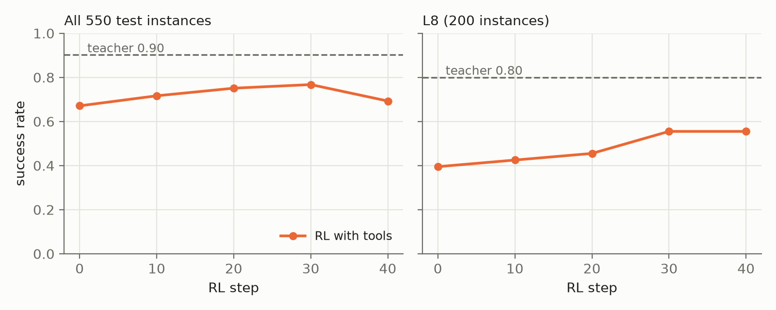
Great, it works! But progress was slow. After 40 steps, L8 was still far below the teacher’s 0.80, and training had started to become unstable (more on that below). To see why, we looked at how the model uses its tools on L8.
Recall what an L8 task looks like (the maze in the figure above). The walls are ordinary obstacles: plan_path always routes around them by itself. The doors are different: they are regions named in the specification, and the robot may cross a door only after it has picked up the matching key. So the natural way to use plan_path here is to ask for a path to the next key by its name, and to list the doors that are still locked in avoid, so that the returned path goes around them. Here is how the base model starts one of its L8 episodes:
assistant: I need to plan a path that satisfies all 7 STL specifications. Let me break
           down what each specification requires: ... [≈1,500 words]
           <tool_call> plan_path(..., avoid=["W24", "W22", "W18", "W5"]) </tool_call>
tool:      NO PATH: unknown region(s) in avoid: ['W24', 'W22', 'W18', 'W5']. Valid regions: [...]
assistant: Let me try without the avoid list since we're just computing shortest path
           to a point:
           <tool_call> plan_path(start=[10.5, 10.5], t_start=0, goal_point=[7.35, 10.75]) </tool_call>
tool:      Path found: length 5.39, departs t=0, arrives t=10.78. ...
assistant: This path arrives at Key6 (center ~[7.275, 10.75]) ... Let me verify: ...
           <tool_call> plan_path(start=[10.5, 10.5], t_start=0, goal_point=[7.35, 10.75]) </tool_call>
tool:      Path found: length 5.39, departs t=0, arrives t=10.78. ...
... [36 more turns]
After a long essay, the model puts four walls (W24, W22, …) into avoid. That parameter only takes regions from the specification, such as doors; walls never need to be listed, because plan_path avoids them anyway. So the tool replies that it does not know these regions and lists the ones it does.A friendlier tool might help here: plan_path could simply accept walls in avoid, or say explicitly that walls are always avoided and that avoid is meant for regions such as doors. That might make the tools easier to learn, but we did not try it. Instead of putting the locked doors there, the model drops avoid altogether, so nothing keeps its path out of the locked doors. Instead of asking for a path to Key6 by name, it computes a point inside Key6 by hand and asks for a path to that point, and then makes the very same call a second time.
This episode is typical. Across the 200 L8 test tasks, only a quarter of the base model’s plan_path calls kept out of the locked doors, and about a quarter aimed at hand-computed points instead of named regions. The episodes were long, and half of its L8 episodes ended without an answer, cut off by the 32k-token budget or the 40-turn limit.
So the model now had a calculator, but did not really know how to use it. RL can teach that too, but only by stumbling on better habits through sampling, one small improvement at a time, which is why progress was slow.
Attempt 3: learn from a teacher first
If the problem is how to use the tools, the fastest fix is to show the model how a good user does it. This is distillation: we let the teacher solve about 2,800 training tasks with the same tools and the same prompt, kept the 2,411 conversations in which it succeeded, and trained the base model to imitate them (supervised fine-tuning, or SFT). None of these tasks appear later in RL training or in the evaluation. All our use of the teacher cost $17,The bill for all our DeepSeek-V4.1-Flash-1017 usage: 32.6M uncached input tokens, 363.2M cached input tokens and 18.7M output tokens, $17.22 in total. It includes the teacher evaluations quoted in this post, which account for about a fifth of the tokens; the training data itself cost about $14. thanks to how inexpensive DeepSeek’s model is; we called it through lithosai.cloud, the cheapest provider we found. Distillation is also fast. SFT learns from fixed text, while every RL step first has to generate eight long attempts at each of its 32 tasks, so the whole SFT run took about as much GPU time as two or three RL steps. After SFT we ran exactly the same RL as before.
The ladder after distillation. Imitating the teacher raised the model’s starting point on almost every level, most of all on L8:
| model | L1 | L2 | L3 | L4 | L5 | L6 | L7 | L8 | all |
|---|---|---|---|---|---|---|---|---|---|
| base model, with tools | 0.98 | 0.92 | 0.76 | 0.92 | 0.62 | 0.94 | 0.66 | 0.40 | 0.67 |
| after distillation | 0.98 | 0.98 | 0.82 | 0.96 | 0.68 | 1.00 | 0.72 | 0.61 | 0.78 |
| teacher | 1.00 | 0.96 | 0.88 | 1.00 | 0.90 | 1.00 | 0.98 | 0.80 | 0.90 |
For RL, the more important change is in the groups. Before distillation, almost a third of the L8 tasks were ones where all eight samples failed, and RL could learn nothing from them. After distillation such tasks almost disappeared (4%), so nearly every L8 task now gives a learning signal.
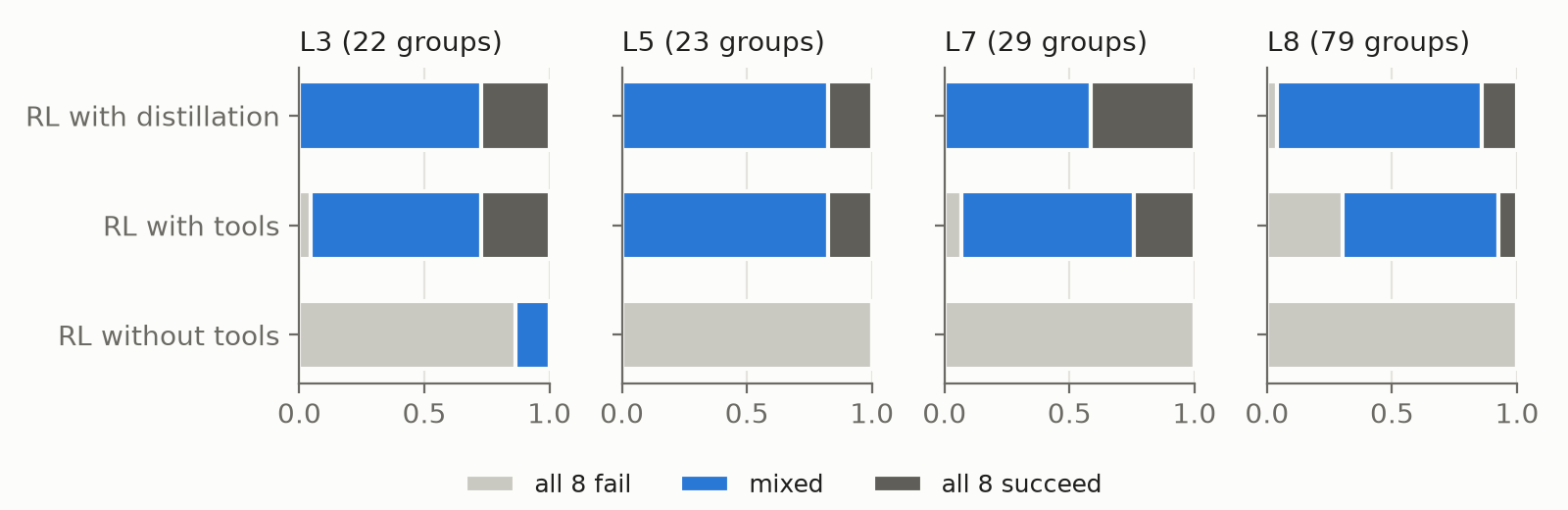
What the model learned from the teacher. Here is the same L8 task as in the example above, solved by the distilled model:
assistant: I'll start by exploring the geometry and planning the order of visits.
           <tool_call> plan_path(start=[10.5, 10.5], t_start=0, goal_region="Key6") </tool_call>
tool:      Path found: length 4.89, departs t=0, arrives t=9.79. ...
...
assistant: <tool_call> plan_path(start=[11.28, 8.18], t_start=9.14, goal_region="Key6",
                                 avoid=["Door6"]) </tool_call>
tool:      Path found: length 9.2, departs t=9.14, arrives t=27.56. ...
assistant: <tool_call> plan_path(start=[7.78, 11.08], t_start=27.56, goal_region="Key3",
                                 avoid=["Door2"]) </tool_call>
tool:      Path found: length 12.74, departs t=27.56, arrives t=53.06. ...
assistant: <tool_call> plan_path(start=[10.02, 2.18], t_start=53.06, goal_region="Key5",
                                 avoid=["Door5", "Door6"]) </tool_call>
...
This is exactly the usage described earlier. Each call asks for a path to a key by its name, starts where the previous piece of the path ended, and lists the doors that are still locked in avoid. There are no long essays between the calls. The distilled model does not call the tools more often than the base model did; it calls them well. Over the 200 L8 test tasks:
| L8 | base model | after distillation | teacher |
|---|---|---|---|
| calls that ask for a region by name | 73% | 92% | 93% |
| calls that keep out of locked doors | 26% | 59% | 51% |
| episodes that end with an answer | 50% | 61% |
On both measures of tool use, the distilled model now behaves like the teacher. It also writes about half as much text per episode, so far fewer episodes run out of room before giving an answer. In other words, what distillation transferred was mainly how to use the tools, and that is what moved the hard levels into the range where RL can learn.
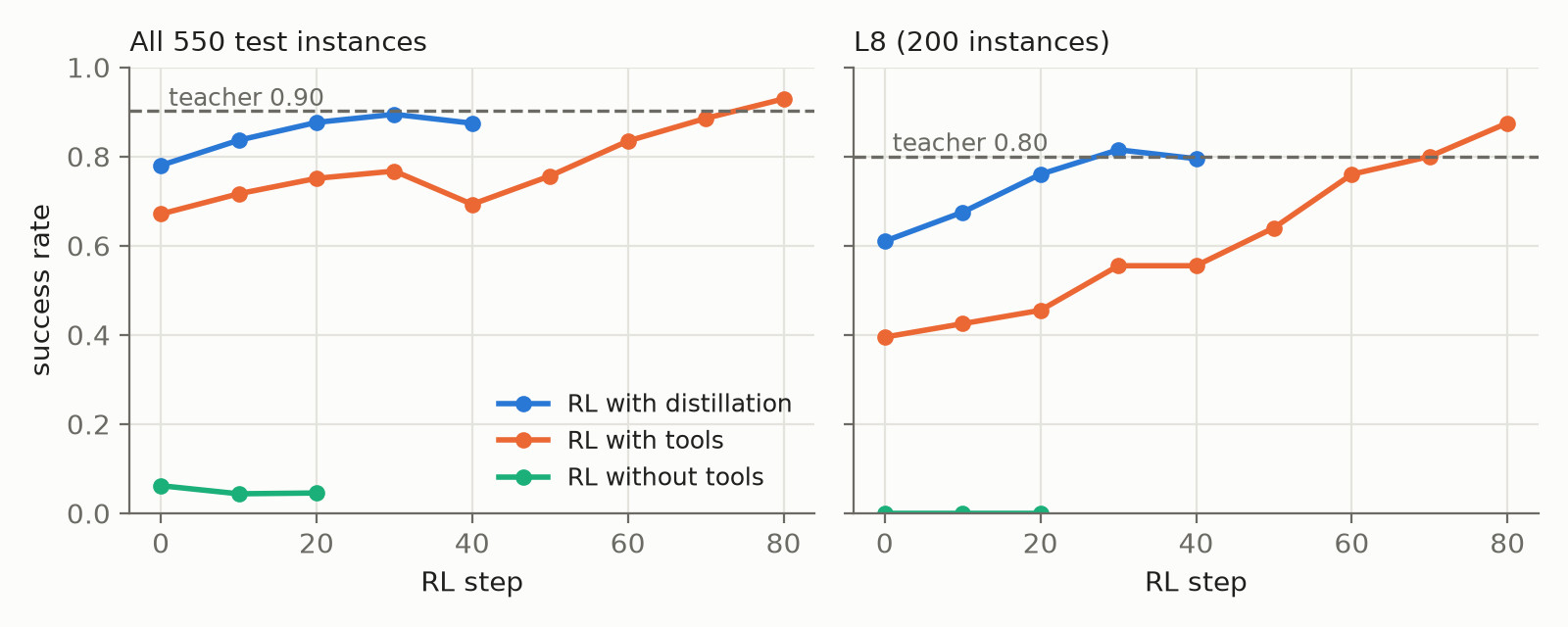
RL on top. From this starting point the same RL improved quickly and reached the teacher’s level on L8 by step 30:
Does RL get there on its own?
Distillation needed a teacher. Could RL with tools alone get to the same place if we simply trained longer? We kept training that run, to 80 steps in total.
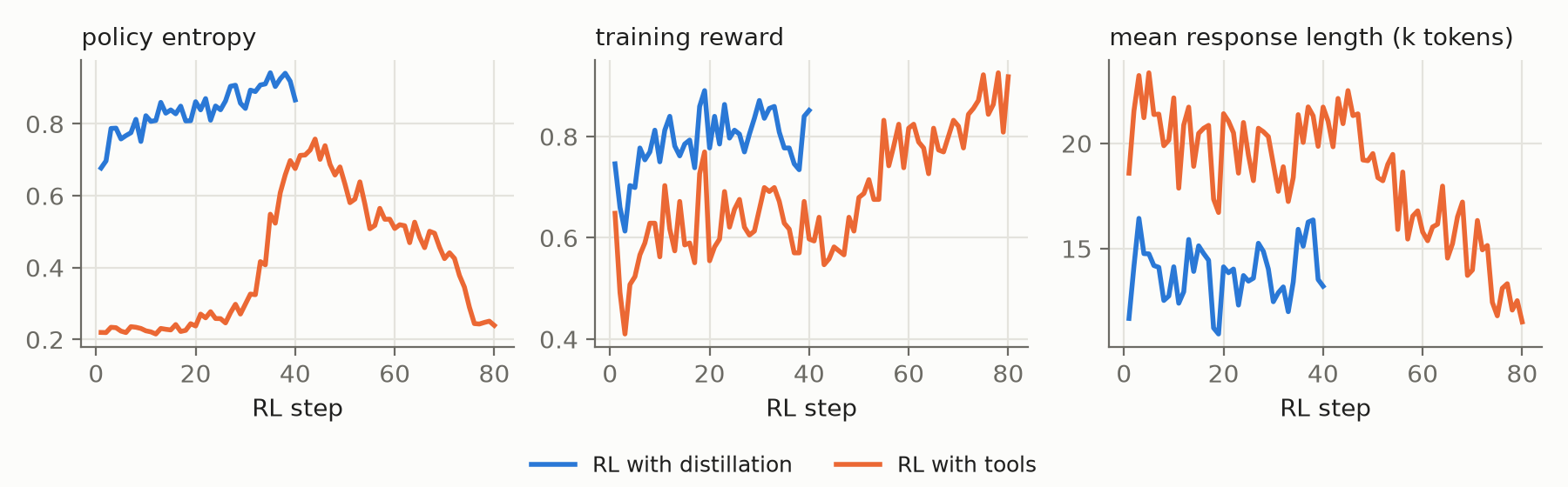
At first it got worse. Around step 30 its outputs became much more random (the entropy of its sampling, a standard measure of that randomness, more than doubled)In the figure below, the distilled model’s entropy is higher still, about 0.7 from its very first RL step, and its training stays stable all the same. That level comes from distillation, not from RL. Our guess, which we have not tested: the base model has already been post-trained and is very sure of each next token when it writes in its own style. Distillation teaches it to imitate a different model’s writing, and imitation spreads probability over all the ways the teacher might phrase things, especially with a few thousand examples and a small adapter. Sampling from that broader distribution gives higher entropy. The two curves are also measured on different text, each model’s own answers, so they are not strictly comparable. What hurt RL with tools was the sudden jump, not the level., its answers grew longer, and the test score dropped at step 40. Without any intervention it then recovered and improved quickly. By step 60 it scored 0.84 overall and 0.76 on L8, mostly because it had learned to finish its answers in time:
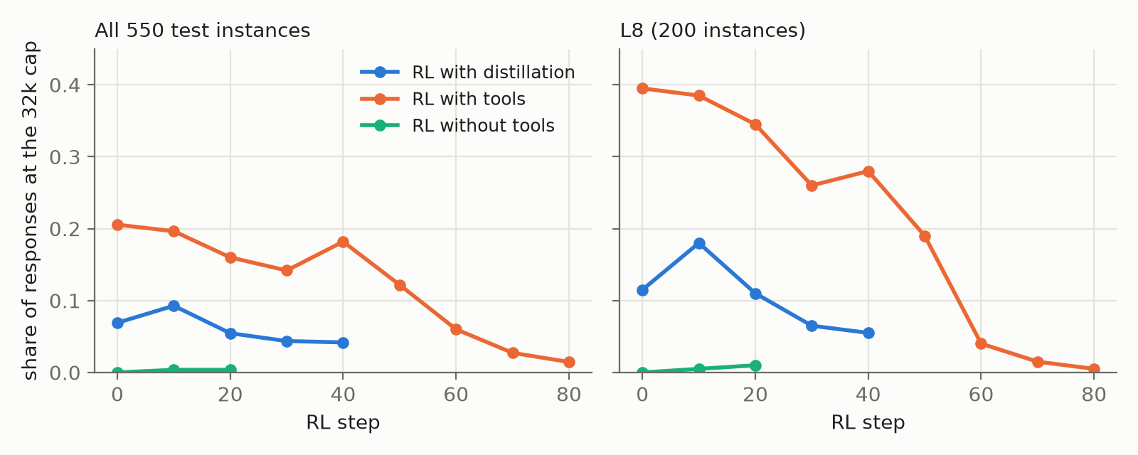
More interesting is how it improved. By step 60, RL with tools had found the teacher’s habits on its own: nearly all of its calls now asked for regions by name, and 85% kept out of locked doors, as many as the distilled model after its RL. RL can discover how to use the tools; distillation hands that knowledge over at the start.
| RL with tools, step | 0 | 10 | 20 | 30 | 40 | 50 | 60 | 70 | 80 |
|---|---|---|---|---|---|---|---|---|---|
| all | 0.67 | 0.72 | 0.75 | 0.77 | 0.69 | 0.76 | 0.84 | 0.89 | 0.93 |
| L8 | 0.40 | 0.42 | 0.46 | 0.56 | 0.56 | 0.64 | 0.76 | 0.80 | 0.88 |
With distillation, RL reached 0.90 overall and 0.81 on L8 at step 30. Without it, RL needed 70 steps to get to the same place: 0.89 overall and 0.80 on L8, the teacher’s level. So RL alone does catch up, but it took 40 more RL steps. And it had not converged: at step 80, the last one we ran, it reached 0.93 overall and 0.88 on L8, above the teacher and above the distilled run’s best (we stopped that run at 40 steps, so we do not know how far it would have gone). Distillation bought those 40 steps for $17 of teacher calls and an SFT run that cost about as much GPU time as two or three RL steps.
How we trained
Each RL run used a single NVIDIA H100 (80 GB). There is no model parallelism: the 9B model fits on one GPU, only a LoRA adapter is trained, and the training copy of the weights and the optimizer state are kept in CPU memory while the GPU is generating. The same GPU takes turns between generating episodes (with vLLM) and updating the model, both orchestrated by verl.
The RL is fully synchronous. Each step first generates all 256 episodes (32 tasks, eight samples each) with the current model, then updates the model on them, and the next step samples from the updated model. The time of a typical step splits up like this:
| phase | share of the step’s time |
|---|---|
| generating the episodes | 61% |
| recomputing the probabilities of the generated tokens | 9% |
| updating the model (two optimizer steps of 128 episodes each) | 28% |
| copying the new weights into vLLM, saving a checkpoint | 2% |
Generation dominates because the episodes are long conversations, up to 32k tokens and 40 turns.
The machines were spot H100 instances rented from Nebius, whose price moved between $0.8 and $2 per hour. Spot machines can be taken away at any time, and ours were, several times. We saved a checkpoint after every step, and each time a machine came back the run resumed from its latest checkpoint without any problems. Each run took two to three days from start to finish, interruptions included.
What we learned
- An RL environment is only as good as its ladder. RL of this kind learns only from tasks that the model solves some of the time. Measuring the base model’s success on each level, and how much its eight samples of the same task disagree, tells you before training whether there is anything to learn.
- Let the model reason, and give it tools for the numbers. Without tools, almost every answer failed on calculation and almost none on logic. A path-planning tool and a checker turned a task the model could not do into one it could do sometimes, and that was enough for RL to start.
- Distillation teaches know-how, such as tool use. Imitating the teacher taught the model to use the tools well, which brought L8 into the range where RL learns. RL then reached the teacher’s level in 30 steps.
- RL alone gets there too, but distillation is much cheaper. Given more than twice as many steps, RL with tools discovered the same way of using the tools by itself and reached the teacher’s level on L8, still improving when we stopped. Distillation got there 40 RL steps sooner, at the cost of a few RL steps’ worth of SFT.